Detecting distributed service abuse with in-stream VPC flow aggregations

The scenario

AWS VPC Flow Logs record every accepted and rejected network flow at the ENI level. In a distributed service abuse attack (credential stuffing, database brute force, API key enumeration), many distinct external IPs each make a small number of connections to the same internal service on the same port. No single source looks alarming in isolation. The signal lives at the destination. 

The raw flow record for one of these rejection events looks like this: 

2 123456789012 eni-0a1b2c3d4e5f60001 45.33.12.87 10.0.1.10 54321 443 6 3 176 1700001020 1700001021 REJECT OK

One event. One rejected SYN. At 500 events per second across a 5-minute attack window, that is 150,000 events. The question you want to answer is: how many sources attempted to reach port 443 on host 10.0.1.10 in the last minute, and is that number anomalous? That question requires one row per destination service per time window, not all 150,000 events individually.

Build the pipeline

1. Create a new pipeline in Splunk Edge Processor.
   1. Set the source to your VPC Flow Log stream.
   2. Set the destination to splunk_indexer.
2. Remove the boilerplate and import the route command to split REJECT and ACCEPT flows into separate aggregation paths.
   import route from /splunk.ingest.commands
3. Start the pipeline and extract all VPC Flow v2 fields from _raw using rex. 
   $pipeline = | from $source 
| rex field=_raw /^(?P<version>\d+)\s+(?P<account_id>\d+)\s+(?P<interface_id>eni-[0-9a-f]+)\s+(?P<srcaddr>[\d.]+)\s+(?P<dstaddr>[\d.]+)\s+(?P<srcport>\d+)\s+(?P<dstport>\d+)\s+(?P<protocol>\d+)\s+(?P<packets>\d+)\s+(?P<bytes>\d+)\s+(?P<start>\d+)\s+(?P<end>\d+)\s+(?P<action>ACCEPT|REJECT)\s+(?P<log_status>OK|NODATA|SKIPDATA)$/ 
4. Use route to open a separate processing path for REJECT flows.
   | route action == "REJECT", [
5. Inside the REJECT branch, use stats with a 1-minute span to produce per-service rejection counts. @maxdelay("2m") holds the window open for up to 2 minutes to absorb late-arriving events before closing and emitting the result. 
     | @maxdelay("2m") stats mode="passthrough" count(action) AS reject_count, 
                                             sum(bytes)    AS rejected_bytes, 
                                             min(packets)  AS min_packets_per_flow, 
                                             max(packets)  AS max_packets_per_flow 
      BY dstaddr, dstport, index, source, sourcetype, host, span(_time, 1m) 
6. Tag the output with a new source type and routing metadata, then send it to the indexer. The closing bracket finalizes the REJECT branch. 
     | eval _raw = dstaddr + " " + dstport, sourcetype="aws:vpc:flow:agg", index="vpc_flow_summary", source="us-east-1", host="ep" 
  | into $destination 
] 
7. ACCEPT flows fall through the route block. Apply the same aggregation to produce a legitimate traffic baseline for comparison at search time. 
   | @maxdelay("2m") stats mode="passthrough" count(action) AS accept_count, 
                                           sum(bytes)    AS accepted_bytes, 
                                           min(packets)  AS min_packets_per_flow, 
                                           max(packets)  AS max_packets_per_flow 
    BY dstaddr, dstport, index, source, sourcetype, host, span(_time, 1m) 
| eval _raw = dstaddr + " " + dstport, sourcetype="aws:vpc:flow:agg", index="vpc_flow_summary", source="us-east-1", host="ep" 
| into $destination; 

This is the complete pipeline: 

import route from /splunk.ingest.commands 
 
$pipeline = | from $source 
| rex field=_raw /^(?P<version>\d+)\s+(?P<account_id>\d+)\s+(?P<interface_id>eni-[0-9a-f]+)\s+(?P<srcaddr>[\d.]+)\s+(?P<dstaddr>[\d.]+)\s+(?P<srcport>\d+)\s+(?P<dstport>\d+)\s+(?P<protocol>\d+)\s+(?P<packets>\d+)\s+(?P<bytes>\d+)\s+(?P<start>\d+)\s+(?P<end>\d+)\s+(?P<action>ACCEPT|REJECT)\s+(?P<log_status>OK|NODATA|SKIPDATA)$/ 
 
| route action == "REJECT", [ 
  | @maxdelay("2m") stats mode="passthrough" count(action) AS reject_count, sum(bytes) AS rejected_bytes, min(packets) AS min_packets_per_flow, max(packets) AS max_packets_per_flow BY dstaddr, dstport, index, source, sourcetype, host, span(_time, 1m) 
  | eval _raw = dstaddr + " " + dstport, sourcetype="aws:vpc:flow:agg", index="vpc_flow_summary", source="us-east-1", host="ep" 
  | into $destination 
] 
| @maxdelay("2m") stats mode="passthrough" count(action) AS accept_count, sum(bytes) AS accepted_bytes, min(packets) AS min_packets_per_flow, max(packets) AS max_packets_per_flow BY dstaddr, dstport, index, source, sourcetype, host, span(_time, 1m) 
| eval _raw = dstaddr + " " + dstport, sourcetype="aws:vpc:flow:agg", index="vpc_flow_summary", source="us-east-1", host="ep" 
| into $destination; 

The mode="passthrough" option on stats retains the original event metadata. The eval that follows replaces _raw with a minimal dstaddr dstport string that serves as a human-readable pointer to the record. The result is an event with a small raw string and all meaningful data in indexed fields, which enables tstats searches against aws:vpc:flow:agg data.

Tune aggregation windows

The @maxdelay and @maxdisk annotations on the stats command control how long and how much the Edge Processor instance holds events in memory before closing a window and emitting the result.

• @maxdelay sets the maximum time the instance will buffer events for a given window. A value of 2m means events will be held for up to 2 minutes to absorb late-arriving events.
  | @maxdelay("2m") stats count(action) AS reject_count ...
• @maxdisk sets a disk space ceiling for buffered window data. If the buffer reaches the limit before @maxdelay expires, the window closes and emits early.
  | @maxdisk("500mb") @maxdelay("2m") stats count(action) AS reject_count ...

Both values can be tuned to match your detection requirements and data volume. Longer delay windows produce more complete aggregations at the cost of increased latency before results reach the index. Larger disk allocations support higher event volumes within a window.

One constraint applies across all pipelines on an instance: memory and disk resources are shared. If multiple pipelines are running concurrently, the combined buffer requirements of all active windows must fit within the physical resources of the instance. Increasing @maxdelay or @maxdisk on high-volume pipelines might require provisioning additional disk or memory on the instance to avoid contention.

For more detail on both annotations see the SPL2 stats command documentation.

Pipeline output

Each 1-minute window closes and emits one event per unique dstaddr/dstport combination. A rejection summary for one service looks like this:

_raw:   10.0.1.10 443
_time:  1781016180
dstaddr:             10.0.1.10
dstport:             443
reject_count:        47
rejected_bytes:      8272
min_packets_per_flow: 1
max_packets_per_flow: 3

Forty-seven raw flow records become one event. The destination service is identified. The attack volume is pre-computed. A min_packets_per_flow of 1 is characteristic of unanswered SYN probes: single-packet connection attempts that never complete a handshake. Because the aggregate values are indexed fields rather than text in _raw, the events are queryable with tstats which bypasses the raw event journal entirely and reads directly from the .tsidx files.

Observed savings

The numbers below are from a representative production deployment. Your results will vary with your traffic mix and destination cardinality, but the categories of savings apply universally.

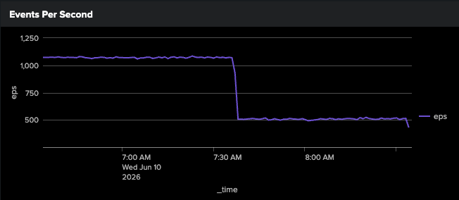
• Indexing rate dropped from approximately 1,000 EPS to 500 EPS after the aggregation pipeline was applied, a 50% reduction in events the indexer had to process.
  
• Indexed data volume dropped from approximately 1 TB/day to 67 GB/day, a 93% reduction. This gain comes directly from replacing large raw flow records with a minimal dstaddr dstport string in _raw. The aggregate values still consume disk as indexed fields, but indexed field storage is significantly smaller than the equivalent raw text.
  

The degree of reduction in both measurements scales with the cardinality of the grouped fields during the aggregation window. The more events that share the same dstaddr/dstport within a 1-minute window, the more that group collapses into a single output event. A distributed attack against one service collapses dramatically. Diverse traffic spread across many unique destinations collapses less. High destination cardinality is the limiting factor.

This also means indexed field-based solutions like this one are best suited to low-cardinality use cases. When destination cardinality is high, the index can accumulate many unique field values and grow larger than a comparable raw-text index would. If you are evaluating this approach for a new data source, measure your destination cardinality first. Where cardinality is naturally low, such as a handful of internal services, the savings are significant. Where it is high, raw indexing might remain the better option.

Search-time final aggregation

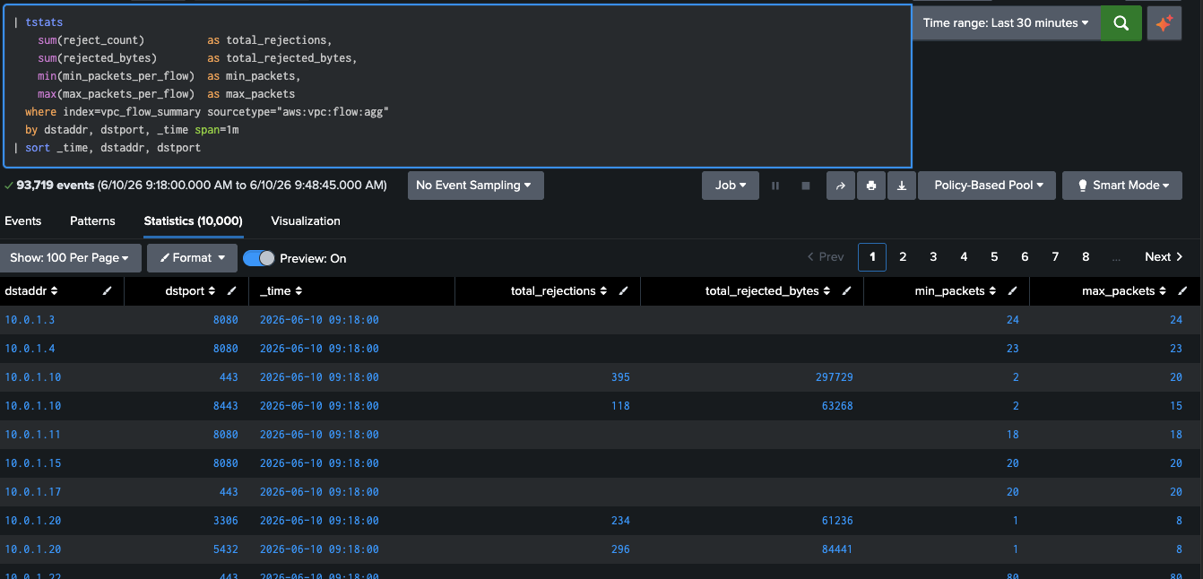
Each Edge Processor instance closes its windows independently. With multiple instances processing the same stream, each emits its own summary for the same time window. A final aggregation pass at search time merges the per-instance results into accurate totals. Because the aggregate values are stored as indexed fields, this pass can use tstats, which reads .tsidx files directly, bypassing the raw event journal for maximum search performance. Use this pattern as the base for all searches against aws:vpc:flow:agg data.

| tstats
    sum(reject_count)          AS total_rejections,
    sum(rejected_bytes)        AS total_rejected_bytes,
    min(min_packets_per_flow)  AS min_packets,
    max(max_packets_per_flow)  AS max_packets
  where index=vpc_flow_summary sourcetype="aws:vpc:flow:agg"
  BY dstaddr, dstport, _time span=1m
| sort _time, dstaddr, dstport

One row per service per minute, regardless of how many instances contributed.

Long-term trend analysis

The 1-minute aggregation windows in vpc_flow_summary are well-suited for real-time detection. For longer lookbacks and historical trend analysis, a scheduled search can roll those per-minute results into hourly summaries. Because the source data is already aggregated and stored as indexed fields, tstats can power the summary population search, keeping it fast and lightweight on every run.

Schedule this search to run hourly with a 2-hour lookback. The wider window absorbs any pipeline or scheduling latency without risk of gaps.

| tstats
    sum(reject_count)           AS total_rejections,
    sum(rejected_bytes)         AS total_rejected_bytes,
    min(min_packets_per_flow)   AS min_packets,
    max(max_packets_per_flow)   AS max_packets
  where index=vpc_flow_summary sourcetype="aws:vpc:flow:agg"
  BY dstaddr, dstport, _time span=1h
| sort _time, dstaddr, dstport
| collect index=vpc_flow_hourly sourcetype="vpc:flow:hourly:summary"

A 7-day window spans 168 hourly buckets per service. Baseline deviation searches, trend charts, and anomaly scoring all run against a small, pre-computed dataset rather than 1-minute windows.

The efficiency compounds at each layer. The pipeline aggregates raw flows at ingest. tstats reads indexed fields to populate the hourly summary. Searches that query the hourly summary read the smallest possible dataset. Each step pays the compute cost one time.

Security detection: Identifying distributed service abuse

This example dashboard provides three panels that together tell the full detection story.

• The first panel is a ranked table of destination host/port pairs showing accepted and rejected flows side by side, with a computed reject ratio and heat-mapped coloring. Services under active attack sort to the top. A high reject ratio on port 443 or 5432 against an internal host is the credential stuffing and database probing signature: many sources, one target, almost no successful connections.
• The second panel is a line chart of rejection volume per service over time, with the top 10 services by volume each rendered as a separate series. A service undergoing a distributed attack produces a sharp, sustained spike that stands out clearly against the flat baselines of unaffected services. The timeline view also reveals the duration and intensity of an attack in a way a static table cannot.
• The third panel compares the current hour against the 7-day hourly average for each service and assigns a severity label. With hourly summary buckets, the 7-day baseline spans 168 buckets. A service whose current-hour rejection count is 3 times or more its hourly average is flagged as Elevated, 5 times is High, and 10 times or above is Critical. The ratio adapts per service, so a naturally noisy host does not generate false positives against a quiet one.

The accept and reject data coexist in the same source type, which makes the two-phase attack pattern visible without joining separate data sources. A service that moves from Critical rejection volume to a sudden spike in accepted connections has likely transitioned from stuffing to successful authentication. That transition is visible in both the table and the timeline.

These panels feed naturally into Splunk Enterprise Security risk-based alerting. The rejection_ratio maps directly to a risk score modifier. A service that crosses the Critical threshold generates a notable; one that sustains elevated ratios across multiple hourly windows escalates the associated asset risk score.

What you gain

Considerations

This technique is one of several options for optimizing high-volume, low-signal data sources. Not every data source benefits from in-stream aggregation. Where individual events carry forensic weight or where cardinality is naturally low, raw indexing remains the right call. Apply this where your data volume and cardinality justify it.

• Your detections and dashboards have to change. Aggregated events land in a new source type (aws:vpc:flow:agg). Existing searches referencing aws:vpc:flow will not see this data. Plan to update knowledge objects, correlation searches, and any Splunk Enterprise Security data models that reference the original source type.
• Each Edge Processor instance aggregates independently. Stats windows close per instance. With multiple instances processing the same stream, a second aggregation pass at search time is required to produce accurate totals. The searches in this article account for this.
• You trade raw events for summaries. The original per-flow records are not retained after aggregation. Splunk Machine Data Lake and the Cisco Data Fabric make it possible to retain raw data in low-cost storage while routing aggregated results to the index, giving you both the summary for fast detection and the raw record for forensic investigation when needed. Note that promoting data from MDL into the index should still apply the same indexing optimizations described here. Low-cost raw storage in MDL does not change what an optimal indexed event looks like. A promotion job that writes full raw flow records into the index lands in the same position as direct raw ingestion. If you are promoting from MDL for detection purposes, apply this aggregation at promotion time rather than treating MDL as a reason to skip it.
• Low destination cardinality is the point. This aggregation groups by destination host and port. It is effective precisely when source IP cardinality is high, which is the defining characteristic of a distributed attack. A per-source aggregation would produce almost no grouping benefit under the same conditions.
• Consider promoting these aggregations to a metrics index. The pipeline output is a time-series metric. Splunk platform metrics indexes store it at lower cost and higher query performance than event indexes. The steps above use an event index to keep the example accessible, but the same data can be written to a metrics index with minor changes.