Converting complex data into metrics with Edge Processor
As an experienced Splunk admin, you have followed data onboarding best practices and have a well-formatted JSON event that you hand off to a data consumer.
Before working through the example in this article, first read Converting logs into metrics with Edge Processor for beginners. In that example, the router metric data represented a set of metrics from a single device connected to a router or gateway. This articles takes a look at a more complicated example.
Rather than a single device being reported, the data from our router can contain an arbitrary number of devices that have connected to that router. The addition of these comma delimited data points and dimensions complicates our data further because now a single event contains multiple unique data points that should be split apart into their own metrics data points rather than being ingested as a single large event.
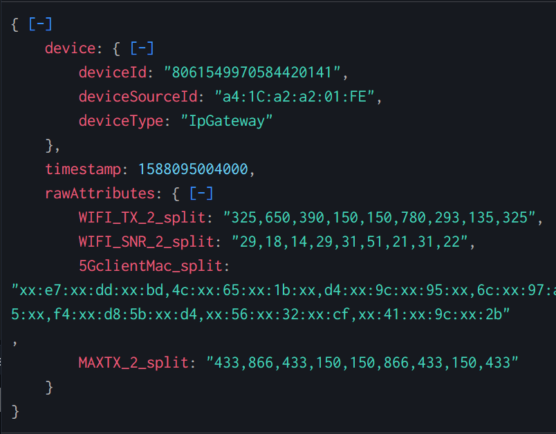
{
  "device": {
    "deviceId": "8061549970584420141",
    "deviceSourceId": "a4:1C:a2:a2:01:FE",
    "deviceType": "IpGateway"
  },
  "timestamp": 1588095004000,
  "rawAttributes": {
    "WIFI_TX_2_split": "325,650,390,150,150,780,293,135,325",
    "WIFI_SNR_2_split": "29,18,14,29,31,51,21,31,22",
    "5GclientMac_split": "xx:e7:xx:dd:xx:bd,4c:xx:65:xx:1b:xx,d4:xx:9c:xx:95:xx,6c:xx:97:ad:xx:92,4c:ef:xx:15:xx:ff,xx:1b:xx:c9:e5:xx,f4:xx:d8:5b:xx:d4,xx:56:xx:32:xx:cf,xx:41:xx:9c:xx:2b",
    "MAXTX_2_split": "433,866,433,150,150,866,433,150,433"
  }
}
The consumer comes back to you, however, with the following complaint:
"These events are from our router. The device field at the top describes the router itself, and then the rawAttributes describes all of the downstream devices that connect to the router and their respective performance values like transmit, receive, and signal to noise values. We want to be able to report on these individual downstream devices over time and associate those individual devices with the router that serviced them as well as investigate the metrics over time. We use this data to triage customer complaints and, over time, improve the resiliency of our network."
This means that multi-device single events must be transformed into distinct values. Worse, every single search that works with this data will need to contain all that same transformation logic, every time. You could do some ingestion-time props and transforms work to pre-format the data, coupled with some summary stats searches to transform these events for consumption. But this solution requires more valuable CPU cycles used, slower search performance overall, additional resource contention, and really just a bad day for the data consumer. You need a better solution.
This article is aimed at more advanced Splunk users and uses a complex data source in the example. For a simplified version of this process, see Converting logs into metrics with Edge Processor for beginners.
Solution
You need to pre-process the data. Building metrics with dimensions for each of the consumer devices will allow them to rely on super fast mstats for their near real-time reporting. With familiar search processing language, you can apply the needed transformations in the stream, before the data is indexed. Doing so removes complexity from the data, reduces search and index time resource consumption, improves data quality, and in the case of this customer, reduces their mean time to identify problems in their environment because they're not waiting for actionable data to be generated.
This example uses data sent from a forwarder to Splunk Edge Processor. You might need to change the data source and applicable Splunk technical add-ons to fit your environment.
- In Splunk Edge Processor, create a pipeline with the following SPL using an appropriate source type and Splunk HEC as the destination.
It’s important to use Splunk HEC as a destination because the output of this pipeline specifically results in metrics-compatible format.
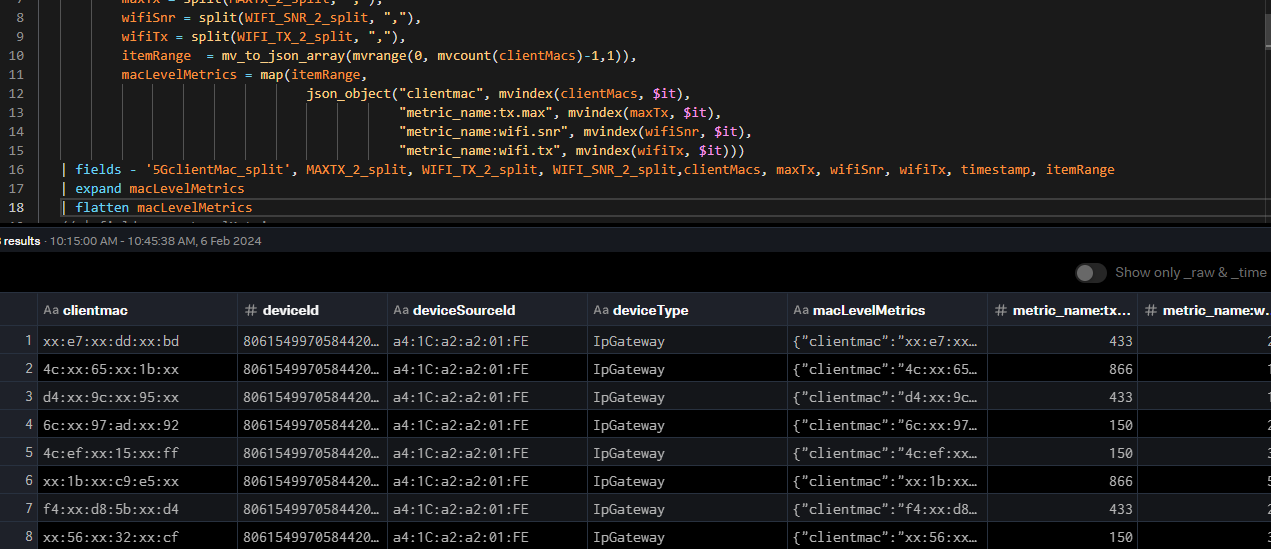
$pipeline = | from $source | flatten _raw | flatten device | flatten rawAttributes | fields - _raw, device, rawAttributes | eval clientMacs = split('5GclientMac_split', ","), maxTx = split(MAXTX_2_split, ","), wifiSnr = split(WIFI_SNR_2_split, ","), wifiTx = split(WIFI_TX_2_split, ","), itemRange = mv_to_json_array(mvrange(0, mvcount(clientMacs)-1,1)), macLevelMetrics = map(itemRange, json_object("clientmac", mvindex(clientMacs, $it), "metric_name:tx.max", mvindex(maxTx, $it), "metric_name:wifi.snr", mvindex(wifiSnr, $it), "metric_name:wifi.tx", mvindex(wifiTx, $it))) | fields - '5GclientMac_split', MAXTX_2_split, WIFI_TX_2_split, WIFI_SNR_2_split,clientMacs, maxTx, wifiSnr, wifiTx, timestamp, itemRange | expand macLevelMetrics | flatten macLevelMetrics | fields - macLevelMetrics | eval _raw = "metric", index="telecom_metrics" | into $destination - Save and apply your pipeline to your Splunk Edge Processor.
- Ensure data is flowing to Splunk Edge Processor.
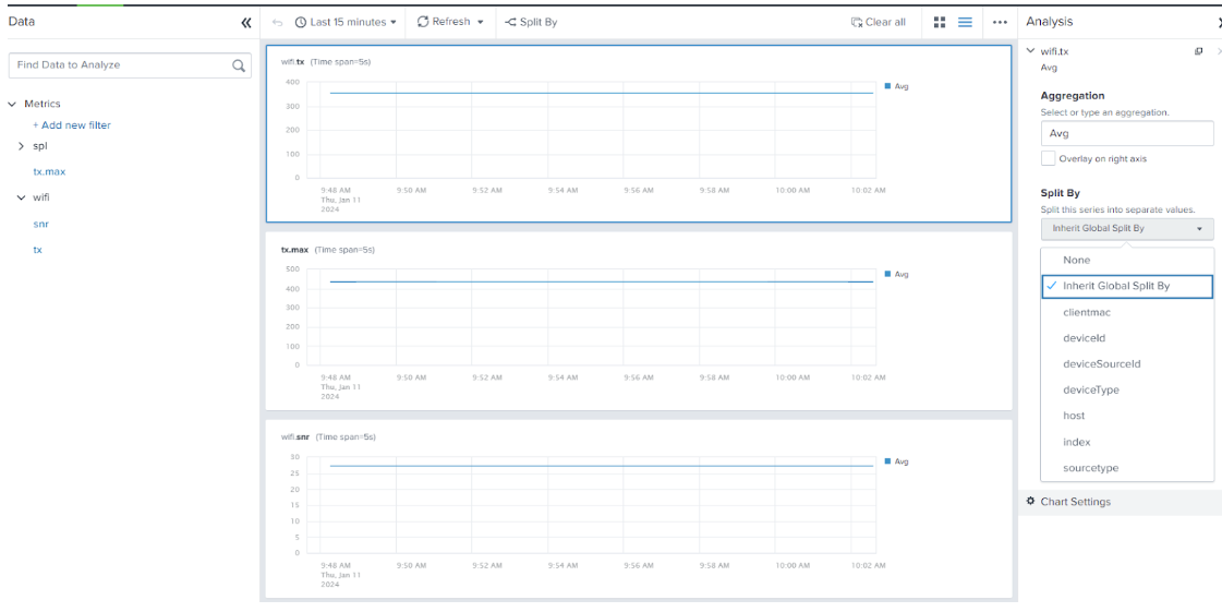
- Using the analytics workbench in Search & Reporting, build charts from these metrics (tx.max, wifi.snr, wifi.tx) to verify that the metrics are available.
Pipeline explanation
The table provides an explanation of what each part of this search achieves. You can adjust this query based on the specifics of your environment.
Throughout the screenshots, some of the preview data is filtered to specific relevant fields for readability.
| SPL | Explanation |
|---|---|
$pipeline = | from $source |
This is how every Splunk Edge Processor pipeline starts. $source is determined by your source data and how you configure partitioning. Here we can see the JSON payload containing the
|
| flatten _raw |
By flattening
|
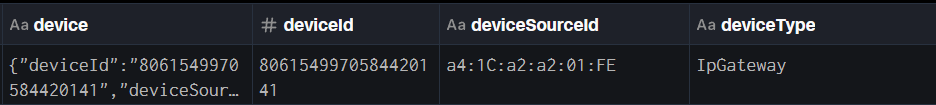
| flatten device |
Since we want all of the fields for the device to become dimensions of our metrics, we can flatten the device field to promote those to the top level as well. We could also use dot (.) notation to access these fields one by one, but if the source data changes and more fields are added,
|
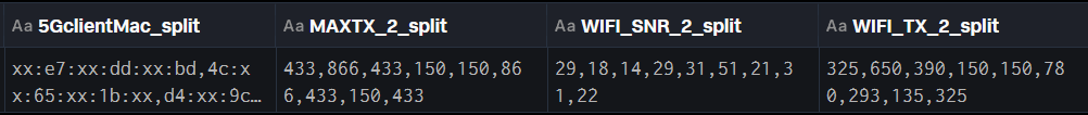
| flatten rawAttributes |
We will also be working with all of the fields in rawAttributes so we may as well bring them to the top using
|
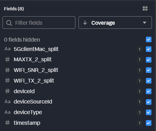
| fields - _raw, device, rawAttributes |
Because we’ve moved all of this field data to the top level, we can remove those original fields from the output. This isn’t strictly necessary at this step, but it keeps our data preview cleaner and easier to work with. You can see that those fields have been removed in the field preview pane. All we have now are the fields we promoted to the top level.
|
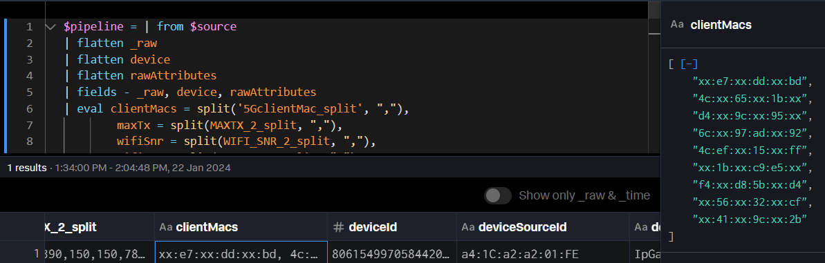
| eval clientMacs = split('5GclientMac_split', ","), |
Our metric data is currently in comma delimited format within the fields. We can use
|
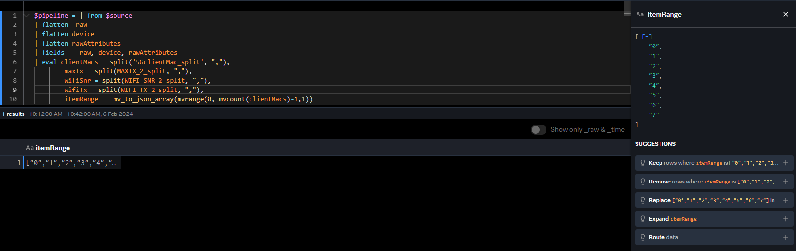
| itemRange = mv_to_json_array(mvrange(0, mvcount(clientMacs)-1,1)), |
We’ll want to iterate through all of the items in each metric array regardless of how large those arrays are. Using
|
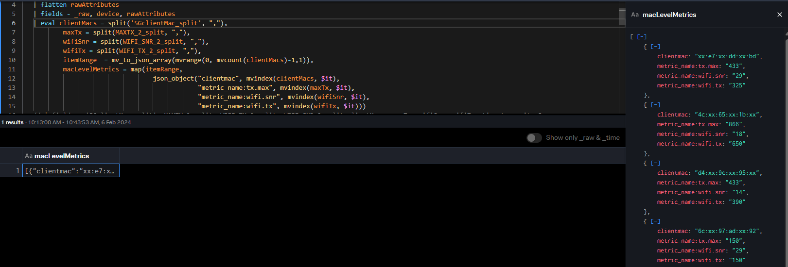
| eval macLevelMetrics = map(itemRange, |
The last big hurdle is going to be “zipping” together each multivalue field into a single object per index number. We can use
|
| fields - '5GclientMac_split', MAXTX_2_split, WIFI_TX_2_split, WIFI_SNR_2_split,clientMacs, maxTx, wifiSnr, wifiTx, timestamp, itemRange |
We’re about to expand this array of mac addresses and metrics, so let’s remove all of the “extra” fields we’ve been working with to keep our data set smaller. If we don’t, all the new events we create will contain all these fields. This will consume more memory and cpu resources. |
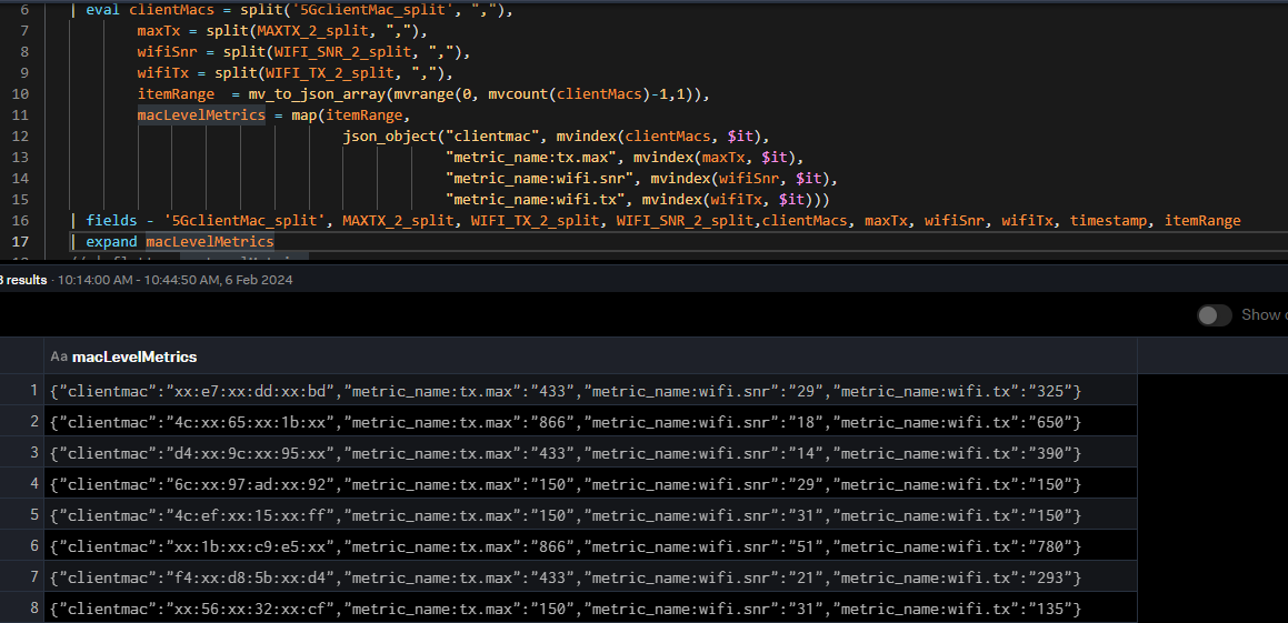
| expand macLevelMetrics |
Now we just need a few minor formatting steps to make the data ready for metrics. In the expand step, we take that array of objects and turn them from a single event into one event per item. You can see we now have 8 events, each representing a different mac address and its associated metrics. Notice how we formatted the field names that are metrics like “metric_name:<field>”. The HEC metric format expects any metric values to be named in this manner.
|
| flatten macLevelMetrics |
As before, we want to promote the values within the
|
| fields - macLevelMetrics |
Now we’ll remove the left-over multivalue field we just expanded. |
| eval _raw = "metric", index="telecom_metrics" |
Finally, referring back to the HEC metrics format, it expects the event data field to be “metric”, and we want to make sure the index we send to is a metrics index. We can do that with a few simple eval commands. Importantly, whatever data is in the _raw field when sent from EP to HEC is stored in the “event” field of the payload. |
| into $destination |
And of course, we need to tell EP where to send this data. $destination will be defined as your Splunk instance as part of the pipeline creation. |

Results
In ten commands, we’ve gone from a single event containing multiple embedded metrics for eight different devices into an expanded metric-based set of statistics, ready to use within seconds of arriving at Edge Processor. At first glance, this may seem like a lot of work. But if you hadn't done this, the user would have had to figure out the best way to split up all those events and that logic would have to be used every single time that data is required. This is a significant barrier removed and it'll make you a hero to your users.
Using the analytics workbench, we can build charts from these metrics and see that the mac address and host dimensions are both available for splitting.
Next steps
These additional Splunk resources might help you understand and implement these recommendations:
- Splunk Docs: About the Edge Processor solution
- Splunk Lantern: Getting started with Splunk Edge Processor
- Splunk Blog: Introducing Edge Processor: Next Gen Data Transformation