Converting logs into metrics with Edge Processor for beginners
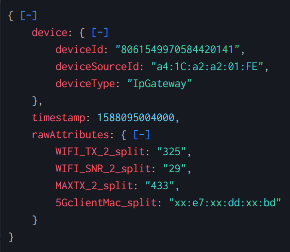
As an experienced Splunk admin, you have followed data onboarding best practices and have a well-formatted JSON event that you hand off to a data consumer.
{
  "device": {
    "deviceId": "8061549970584420141",
    "deviceSourceId": "a4:1C:a2:a2:01:FE",
    "deviceType": "IpGateway"
  },
  "timestamp": 1588095004000,
  "rawAttributes": {
    "WIFI_TX_2_split": "325",
    "WIFI_SNR_2_split": "29",
    "MAXTX_2_split": "433",
    "5GclientMac_split": "xx:e7:xx:dd:xx:bd"
  }
}
The consumer comes back to you, however, with the following complaint:
"These events are from our router. The device field at the top describes the router itself, and then the rawAttributes describes a specific unit that connects to the router and its respective performance values like transmit, receive, and signal to noise values. We want to be able to report on these metrics over time and associate those metrics with the router that serviced the unit. We use this data to triage customer complaints and over time, improve the resiliency of our network."
While the raw text-based data can be fairly easily aggregated using commands like stats in a normal splunk log index, since the data points are all numeric and there’s a relatively small number of dimensions, using a Splunk metrics index and mstats might offer a more performant metrics reporting experience. Let’s explore how we can build metrics from these logs and put them into a metrics index using Splunk Edge Processor.
This article uses a simple logs-to-metrics example. For a more advanced example of this process using a complex data source, see Converting complex data into metrics with Edge Processor.
How to use Splunk software for this use case
Using Splunk Edge Processor, you can extract the metrics fields and associate all of the textual data as the metric dimensions. This will allow you and your customers to leverage super-fast mstats for near real-time reporting. With familiar search processing language, you can apply the needed transformations in the stream, before the data is indexed. Doing so removes complexity from the data, reduces search and index time resource consumption, improves data quality, and in the case of this customer, reduces their mean time to identify problems in their environment because they're not waiting for actionable data to be generated.
This example uses data sent from a forwarder to Splunk Edge Processor. You might need to change the data source and applicable Splunk technical add-ons to fit your environment.
- In Splunk Edge Processor, create a pipeline with the following SPL using an appropriate source type and Splunk HEC as the destination.
It’s important to use Splunk HEC as a destination because the output of this pipeline specifically results in metrics-compatible format.
$pipeline = | from $source | flatten _raw | flatten device | flatten rawAttributes | fields - _raw, device, rawAttributes | rename '5GclientMac_split' as 'mac', 'MAXTX_2_split' as 'metric_name:tx.max', 'WIFI_SNR_2_split' as 'metric_name:wifi.snr', 'WIFI_TX_2_split' as 'metric_name:wifi.tx' | eval _raw = "metric", index="telecom_metrics" | into $destination - Save and apply your pipeline to your Splunk Edge Processor.
- Ensure data is flowing to Splunk Edge Processor.
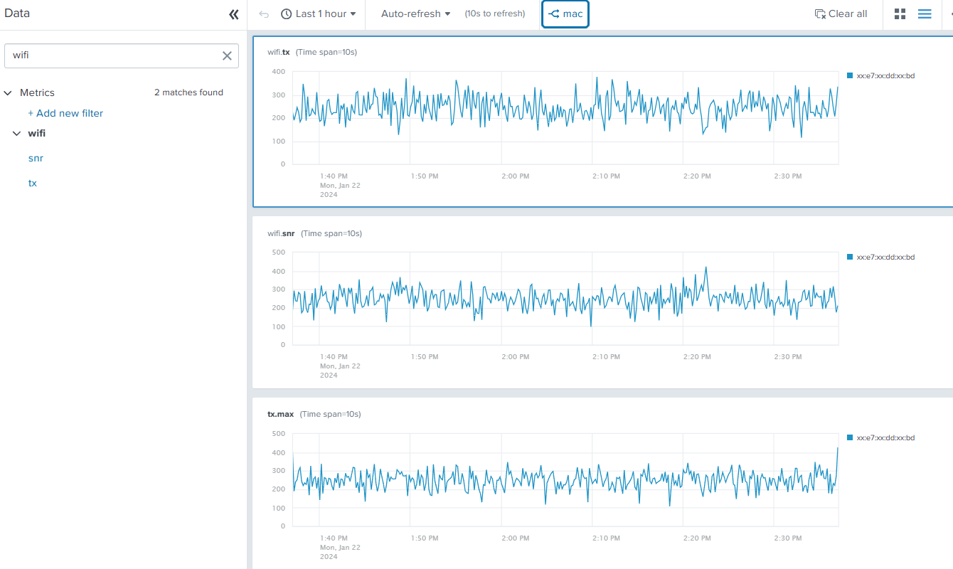
- Using the analytics workbench in Search & Reporting, build charts from these metrics (tx.max, wifi.snr, wifi.tx) to verify that the metrics are available.
Pipeline explanation
The table provides an explanation of what each part of this pipeline achieves. You can adjust this query based on the specifics of your environment and data.
Throughout the screenshots, some of the preview data is filtered to specific relevant fields for readability.
| SPL | Explanation |
|---|---|
$pipeline = | from $source |
This is how every Splunk Edge Processor pipeline starts.
|
| flatten _raw |
By flattening
|
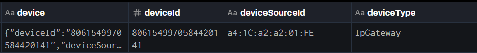
| flatten device |
Because we want all of the fields for the device to become dimensions of our metrics, we can flatten the device field to promote those to the top level as well. We could also use dot (.) notation to access these fields one by one, but if the source data changes and more fields are added, flatten captures any additional new fields automatically.
|
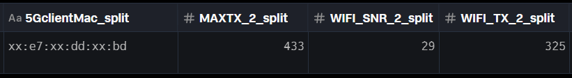
| flatten rawAttributes |
We will also be working with all of the fields in
|
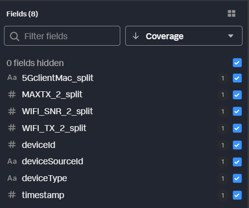
| fields - _raw, device, rawAttributes |
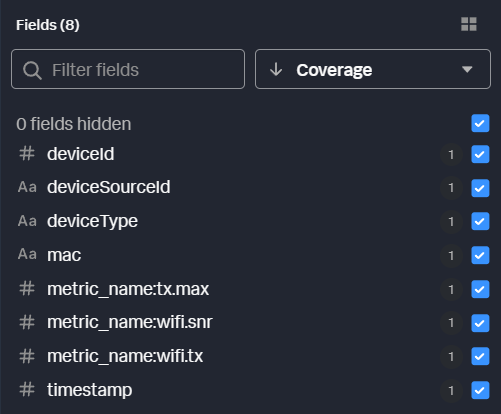
Because we’ve moved all of this field data to the top level, we can remove those original fields from the output. This isn’t strictly necessary at this step, but it keeps our data preview cleaner and easier to work with. You can see that those fields have been removed in the field preview pane. All we have now are the fields we promoted to the top level.
|
| rename '5GclientMac_split' as 'mac', |
All that’s left is to rename the original fields to metrics compatible field names. The client mac address will be a dimension, and the remaining fields will become the metrics we want to use. Any fields that should become metrics are prefixed with “metric_name:”. Any other fields in the data will automatically become dimensions. To understand field naming better, refer to the HEC Metrics format in Splunk Help.
|
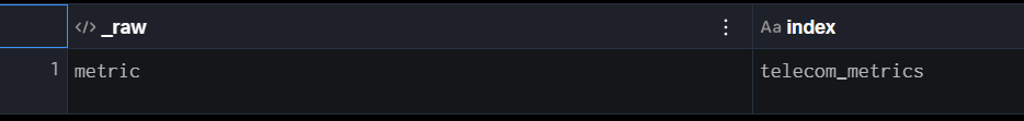
| eval _raw = "metric", index="telecom_metrics" |
Finally, referring back to the HEC metrics format, it expects the event data field to be “metric”, and we want to make sure the index we are sending to is a metrics index. We can do that with a few simple evals. Importantly, whatever data is in the
|
| into $destination |
And of course, we need to tell Splunk Edge Processor where to send this data. $destination is defined as your Splunk instance as part of the pipeline creation. |

Results
In six commands, we’ve gone from a single, text based event containing multiple embedded metrics and dimensions to a Splunk HEC payload that delivers those into a metrics index ready to use within seconds of arriving at Splunk Edge Processor. Now you and your users can leverage the analytics workbench, mstats, and other metrics-specific capabilities to rapidly build and consume these metrics data. In this example the original payload is JSON, but the same process holds true for unstructured data as well. Notably, unstructured, raw data that is converted to numeric/dimensioned metrics will have an even more significant impact when compared to raw search-time analytics.
Next steps
These additional Splunk resources might help you understand and implement these recommendations:
- Splunk Help: About the Edge Processor solution
- Splunk Lantern: Getting started with Splunk Data Management Pipeline Builders
- Splunk Blog: Introducing Edge Processor: Next Gen Data Transformation